STATISTICS for Class 11 MATHS

Hello bachcho, statistics aap kafi pehle se padhte aa rahe hai. Toh aapko iske bare mai thoda bahot idea to zarur hoga ki hum statistics mai data ke bare mai padhte hai. Well statistics maths ka ek bahot important branch hai. Statistics mai jo hum data collect karte hai uska use hamesha kisi na kisi specific purpose ke liye hota hai. Hum uss data ko analyse aur interpret karke kisi decision tak pahuchte hai. Humne earlier classes mai data ko graphically aur tabular form mai represent karna seeka tha. Abh aap suppose kare ki hume ek class ke baccho ki height find out karni hai to hum statistics ka use karke sab baccho ki height find out kar lenge. Agar koi humse puchega ki iss class ke bachho ki height kitni hai to hum unko bolenge ki average height itni hai. Toh ye jo average word use hua hai iske concept ko hum mean kehte hai.
Mean ke baad hum median ko find out karenge. The median is the middle number in a sorted ascending or descending.
If the number of observations is odd, then the median is ${\left(\frac{n+1}{2}\right)}^{th}$ observation.
If the number of observations is even, then median is the mean of ${\left(\frac{n}{2}\right)}^{th}$ and ${(\frac{n}{2}+1)}^{th}$ observations.
These are the measures of central tendency :-

• Mean
• Median
• Mode.

Statistics can be defined as the collection, presentation, classification, analysis, and interpretation of quantitative data.

Statistics help in providing data as well as tools to analyze the data. Statistical knowledge helps you use the proper methods to collect the data, employ the correct analyses, and effectively present the results. An example of statistics is a report of numbers saying how many followers of each religion there are in a particular country.

Karl Pearson was a british statistician and was the founder of mathematical statistics.

The dispersion or scatter in a data is measured on the basis of the observations and the types of the measure of central tendency, used there. There are following measures of dispersion :-
(i) Range
(ii) Quartile deviation
(iii) Mean deviation
(iv) Standard deviation.
Iss chapter mai hum sabhi measures of dispersion ko padhenge except quartile deviation.

Range ko samjhne ke liye sabse pehle hum ek example lete hai .
Humne class ke sabhi baccho ke marks ka data collect kiya hai.
Class A : $30,91,10,64,42,80,30,7,97,71,23,34,67.$
Abh hume range nikalne ke liye maximum value mai se minimum value ko minus karna hoga. Toh yaha par maximum value $97$ hai aur minimum value $7$.
So,
Range = Maximum value – Minimum value.
Range = $97-7=90.$
The range of data gives us a rough idea of variability or scatter but does not tell about the dispersion of the data from a measure of central tendency.

In statistics, deviation means the difference between the observed value and the expected value of a variable. In simple words, the deviation is the distance from the centre point. The centre point can be median, mean, or mode. Similarly, the mean deviation or the mean absolute deviation is used to compute how far the values fall from the middle of the data set. Some of the deviations will be negative and some positive. Thus, the sum of deviations may vanish.
Mean deviation for ungrouped data
Let $n$ observations be $x_1,x_2,x_3,.....,x_n.$
The following steps are involved in the calculation of mean deviation about mean or median :
Step $1$ :- Calculate the measure of central tendency about which we are to find the mean deviation. Let it be $‘a’.$
Step $2$ :- Find the deviation of each $x_i$ from $a,$ i.e., $x_1-a,x_2-a,x_3-a,......,x_n-a.$
Step $3$ :- Find the absolute values of the deviations, i.e., drop the minus sign $(–),$ if it is there, i.e., $|x_1-a|,|x_2-a|,|x_3-a|,.....,|x_n-a|.$
Step $4$ :- Find the mean of the absolute values of the deviations. This mean is the mean deviation about $a,$ i.e.,
M.D. $\left(a\right)$ $=\frac{{\sum }_{i=1}^n|x_i-a|}{n}$
M.D. $\left(\overline{x}\right)$ = $\frac{1}{n}\sum _{i=1}^n|x_i-\overline{x}|,$ where $\overline{x}=$ Mean
M.D. $\left(M\right)$ $=\frac{1}{n}\sum _{i=1}^n|x_i-M|,$ where $M=$ Median.
Mean deviation for grouped data We know that data can be grouped into two ways :
$\left(a\right)$ Discrete frequency distribution,
$\left(b\right)$ Continuous frequency distribution.
Toh chalo mean deviation ko find out karne ke liye hum inn dono methods ko discuss karte hai.
$\left(a\right)$ Discrete frequency distribution :- A discrete distribution is one in which the data can only take on certain values.

$\left(i\right)$ Mean deviation about mean Sabse pehle hum mean $\left(\overline{x}\right)$ nikalenge by using the formula,
$\left(\overline{x}\right)=\frac{{\sum }_{i=1}^n{x}_i{f}_i}{{\sum }_{i=1}^n{f}_i}=\frac{1}{N}\sum _{i=1}^n{x}_i{f}_i,$
where $\sum _{i=1}^n{x}_i{f}_i$ denotes the sum of the products of observations $x_i$ with their respective frequencies $f_i$ and $N=\sum _{i=1}^n{f}_i$ is the sum of the frequencies. Then, we find the deviations of observations $x_i$ from the mean $\overline{x}$ and take their absolute values, i.e., $|x_i-\overline{x}|$ for all $i=1,2,...,n.$
After this, find the mean of the absolute values of the deviations, which is the required mean deviation about the mean. Thus
$M.D.\left(\overline{x}\right)=\frac{{\sum }_{i=1}^n{f}_i|x_i-\overline{x}|}{{\sum }_{i=1}^n{f}_i}=\frac{1}{N}\sum _{i=1}^n{f}_i|x_i-\overline{x}|$
$\left(ii\right)$ Mean deviation about median To find mean deviation about median, we find the median of the given discrete frequency distribution. For this the observations are arranged in ascending order. After this the cumulative frequencies are obtained.
After finding median, we obtain the mean of the absolute values of the deviations from median.Thus,
$M.D.\left(M\right)=\frac{1}{N}\sum _{i=1}^n{f}_i|x_i-M|$
$\left(b\right)$ Continuous frequency distribution :- A continuous frequency distribution is a series in which the data are classified into different class-intervals without gaps along with their respective frequencies.

$\left(i\right)$ Mean deviation about mean :- Hum jab continuous frequency distribution ka mean find out karte hai toh hum ye assume karte hai that the frequency in each class is centred at its mid-point. Hum yaha par har class ka mid point bhi find out karte hain aur discrete frequency distribution ka use karte hai mean deviation ko nikalne ke liye.
For mid point you have to take a look on this formula,
$\frac{\text{Upper limit + Lower limit}}{2}$
Mean deviation about mean $M.D.\left(\overline{x}\right)=\frac{1}{N}\sum _{i=1}^n{f}_i|x_i-\overline{x}|$
Shortcut method for calculating mean deviation about mean
To calculate mean deviation about mean by shortcut method,
First take an appropriate 'Assumed Mean' $A.$
calculate the sum of the frequencies, $\sum _{i=1}^n{f}_i.$
calculate $\sum _{i=1}^n{f}_i{d}_i$, where, $d_i=\frac{x_i-A}{h}$ and $h$ is the common factor.
Then, the mean $\left(\overline{x}\right)$ by step-deviation method is given by
$\overline{x}=A+\frac{{\sum }_{i=1}^n{f}_i{d}_i}{N}\times h$
where $N=f_i$
$\left(ii\right)$ Mean deviation about median :- The process of finding the mean deviation about median for a continuous frequency distribution is similar as we did for mean deviation about the mean.
Sabse pehle aapko median find out karna padega aur median ko hum $M$ se denote karte hain aur median ko nikalne ke liye hum iss formula ka use karte hain.
Median $\left(M\right)=l+\frac{\frac{N}{2}-C}{f}\times h$
$l=\text{lower limit}$
$\frac{N}{2}=\text{selected class interval divide by 2}$
$C=\text{cumulative frequency}$
$f=\text{frequency}$
$h=\text{common factor}$
Thus, Mean deviation about median is given by
M.D. $\left(M\right)=\frac{1}{N}\sum _{i=1}^n{f}_i|x_i-M|$

$\left(i\right)$ The median is not a true representative of a central tendency in a series where the degree of variability. So the mean deviation calculated the about the median for a such a series is not completely reliable.
$\left(ii\right)$ The sum of the deviations from the mean (ignoring the minus signs) is more than the sum of the deviations from median. So, the mean deviation about the mean is not very scientific. Hence, in some cases, mean deviation may not give satisfactory results.
$\left(iii\right)$ The mean deviation is calculated on the basis of absolute values of the deviations. Hence it cannot be subjected to further algebraic treatment.

Find the mean deviation about the mean for the following data :
ltimg src="https://d10lpgp6xz60nq.cloudfront.net/physics_images/RSA_MATH_XI_C30_S01_004_Q01.png" width="80%"gt

We have
$N=\stackrel{6}{\underset{i=1}{\Sigma }}{f}_i=(6+8+15+25+8+4)=66.$
$\overline{x}=\frac{\stackrel{6}{\underset{i=1}{\Sigma }}{f}_i{x}_i}{N}=\frac{(6\times 3)+(8\times 5)+(15\times 7)+(25\times 9)+(8\times 1)+(4\times 13)}{66}$
$=\frac{528}{66}=8.$
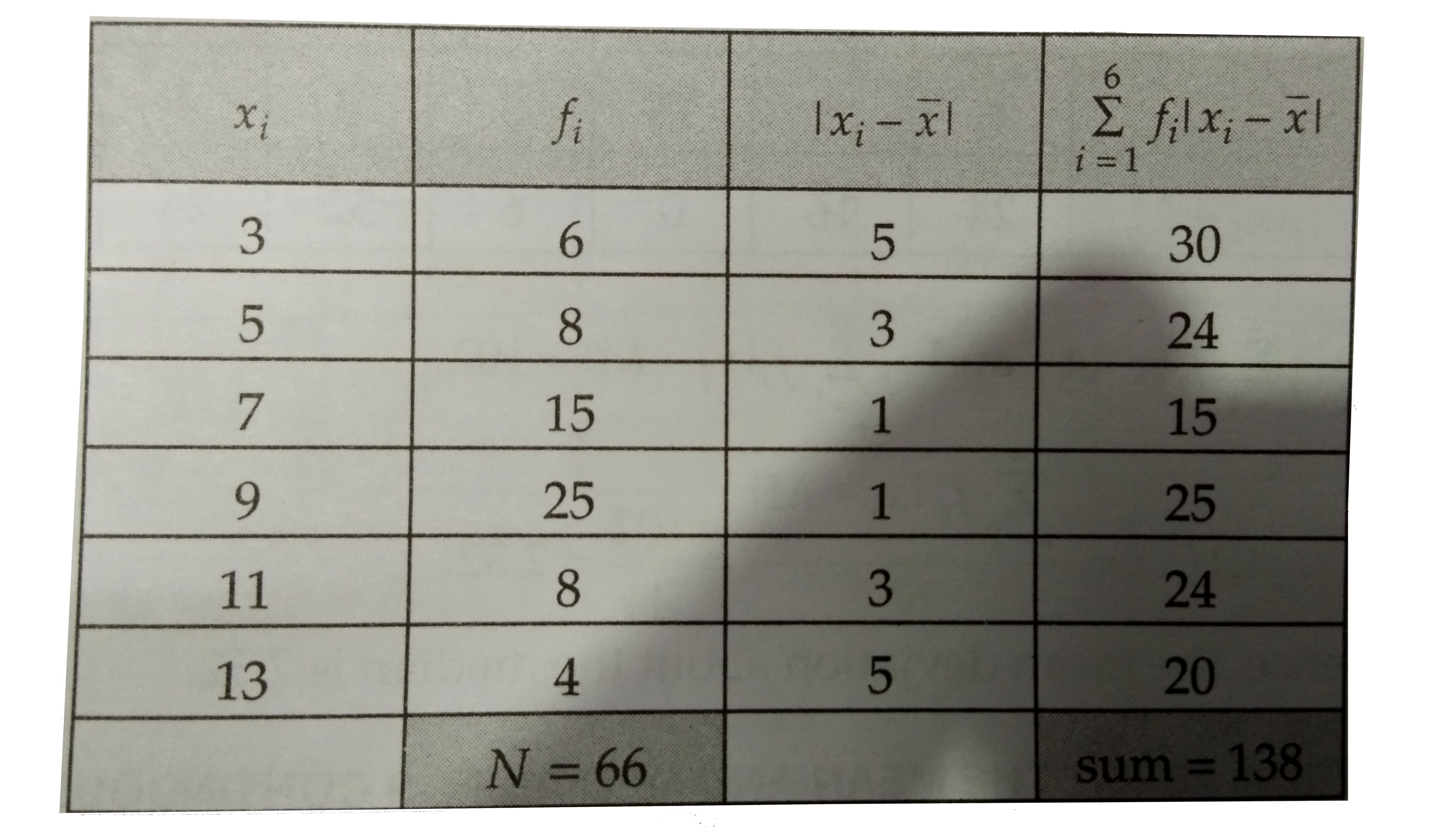
Now, we prepare the table given below :

$\therefore MD\left(\overline{x}\right)=\frac{\stackrel{6}{\underset{i=1}{\Sigma }}{f}_i|x_i-\overline{x}|}{N}=\frac{138}{66}=\frac{23}{11}=209.$
Hence, mean deviation about the mean $=2.09.$

Calculate the mean deviation about the median for the following data :
ltimg src="https://d10lpgp6xz60nq.cloudfront.net/physics_images/RSA_MATH_XI_C30_S01_008_Q01.png" width="80%"gt

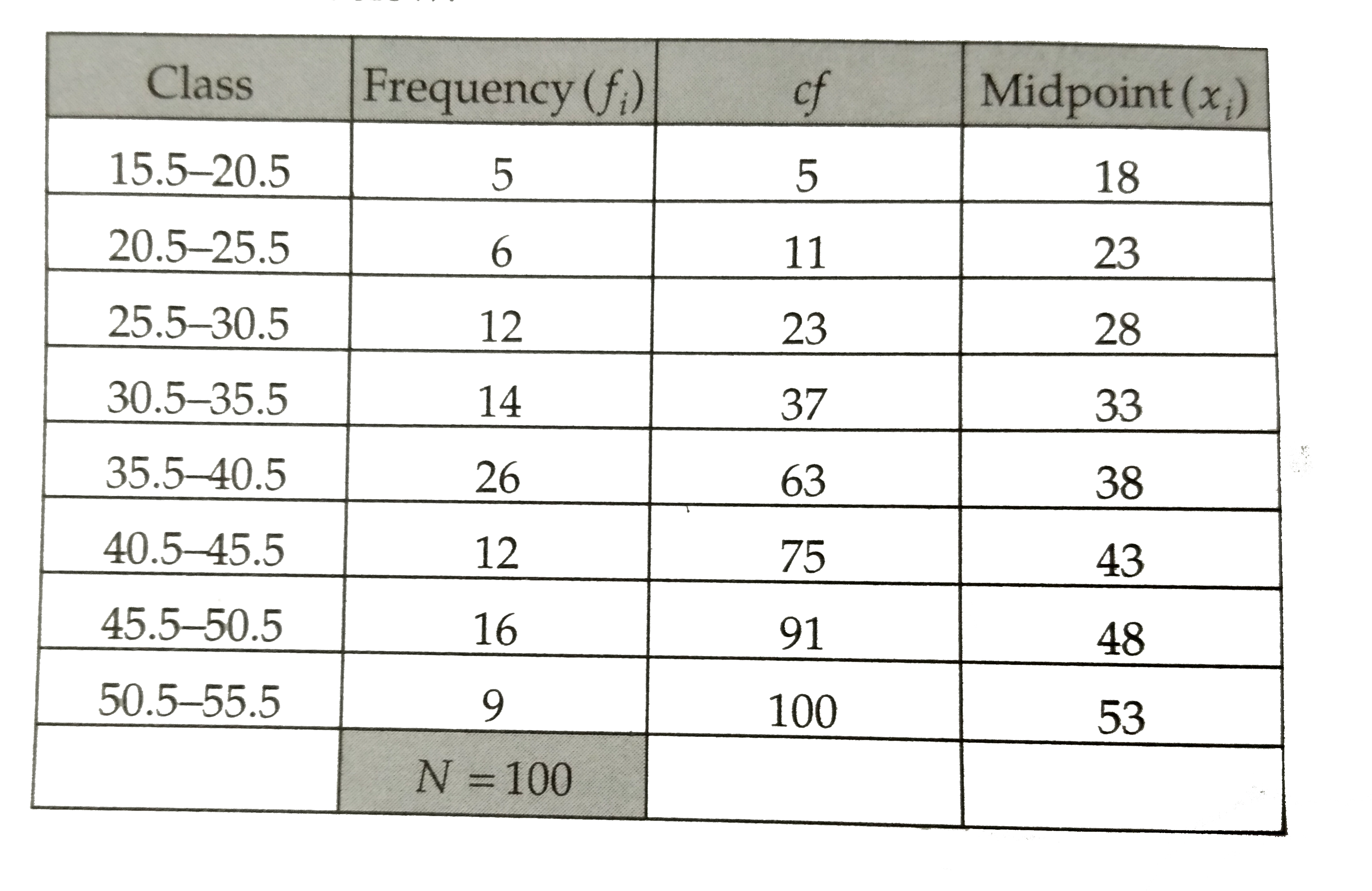
Converting the given series into an exclusive series, we prepare the table, given below :

Thus N=100 and therefore, $\frac{N}{2}=50$
$\Rightarrow medians35.5-40.5$
$\Rightarrow L=35.5,f=26,h=5\text{and}c=37.$
$\therefore \text{median}=L+\frac{(\frac{N}{2}-c)}{f}\times h$
$=\{35.5+\frac{(50-37)}{26}\times 5\}=(35.5+2.5)=38.$
Thus, M=38.
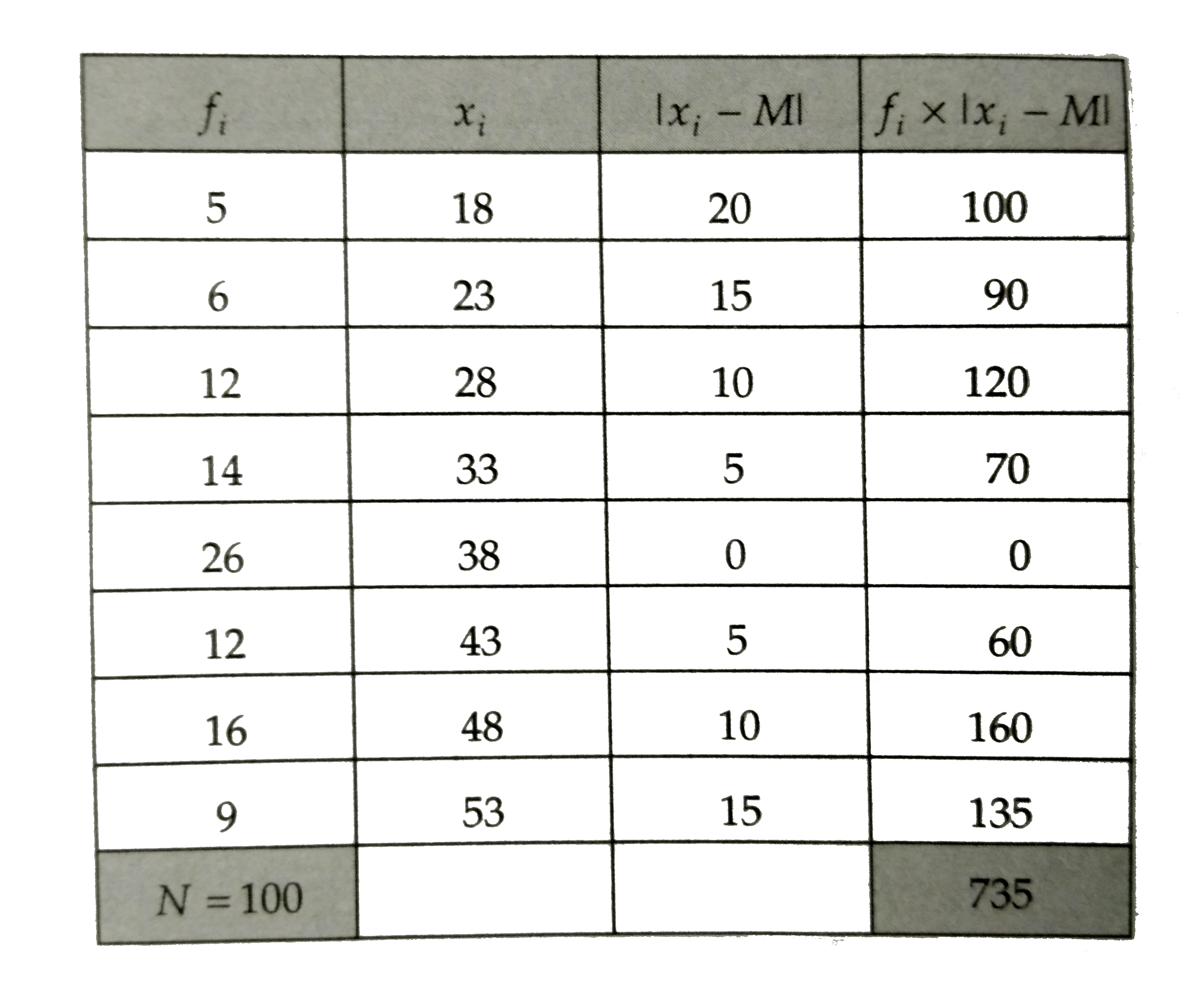
Now, we prepare the table given below :

Thus, $\Sigma f_i\times |x_i-M|=735\text{and}N=100.$
$\therefore MD\left(M\right)=\frac{\Sigma f_i\times |x_i-M|}{N}=\frac{735}{100}=7.35.$
Hence, the mean deviation about the median is 7.35.

Find the mean deviation about the median for the data : $36,72,46,42,60,45,53,46,51,49.$

$36,2,45,46,46,49,51,53,60,72$
median = $\frac{5th+6th}{2}$
$=\frac{46+49}{2}=\frac{95}{2}=47.5$
median deviation =$\frac{\sum |x_i-47.5|}{10}$
$=\frac{11.5+5.5+2.5+1.5+1.5+1.5+3.5+5.5+12.5+24.5}{10}$
$=\frac{5+65}{10}=7$
answer

Variance and Standard Deviation are the two important measurements in statistics.
Variance is a measure of how data points vary from the mean, whereas standard deviation is the measure of the distribution of statistical data.
The basic difference between both is standard deviation is represented in the same units as the mean of data, while the variance is represented in squared units.
Variance According to layman’s words, the variance is a measure of how far a set of data are dispersed out from their mean or average value. It is denoted as $\text{'}{\sigma }^2\text{'}$
Variance Formula:
${\sigma }^2=\frac{1}{n}\sum _{i=1}^n{(x_i-\overline{x})}^2$
Here,
${\sigma }^2=\text{variance}$
$n=\text{Number of observations in population}$
$x_i=\text{ith observation in the population}$
$\overline{x}=\text{mean}$
Standard Deviation Standard deviation is the measure of dispersion of a set of data from its mean and square-root of the variance is called standard deviation. Therefore, the standard deviation, usually denoted by $\sigma$ , is given by
$\sigma =\sqrt{\frac{1}{n}\sum _{i=1}^n{(x_i-\overline{x})}^2}$
Standard deviation of a discrete frequency distribution : Let the given discrete frequency distribution be

$\left(\sigma \right)=\sqrt{\frac{1}{N}\sum _{i=1}^n{f}_i{(x_i-\overline{x})}^2}$
where, $N=\sum _{i=1}^n{f}_i$
This formula will also use in continuous frequency distribution.
Shortcut method to find variance and standard deviation
Kafi baar hume discrete series mai $x_i$ ki value or continuous distribution mai different class ke mid point yani $x_i$ ki value ko nikalne ke liye bahot long calculations karni padti hai aur jo ki bahot zyada time consuming hai. By using step-deviation method, it is possible to simplify the procedure.
Let the assumed mean be $‘A’$ and the scale be reduced to $\frac{1}{h}$ times ($h$ being the width of class-intervals). Let the step-deviations or the new values be $y_i$
i.e. $y_i=\frac{x_i-A}{h}$ or $x_i=A+h{y}_i$.........$\left(1\right)$
We know that $\overline{x}=\frac{{\sum }_{i=1}^n{f}_i{x}_i}{N}$ .......$\left(2\right)$
Replacing $x_i$ from $\left(1\right)$ in $\left(2\right),$ we get
$\overline{x}=\frac{{\sum }_{i=1}^n{f}_i(A+h{y}_i)}{N}$
$=\frac{1}{N}(\sum _{i=1}^n{f}_{i}A+\sum _{i=1}^{n}h{f}_i{y}_i)=\frac{1}{N}(A\sum _{i=1}^n{f}_i+h\sum _{i=1}^n{f}_i{y}_i)$
$=A.\frac{N}{N}+h\frac{{\sum }_{i=1}^n{f}_i{y}_i}{N}$ (because $\sum _{i=1}^n{f}_i=N$)
Thus, $\overline{x}=A+h\overline{y}$.......$\left(3\right)$
Variance of the variable $x,$ ${\sigma }^{2}x=\frac{1}{N}\sum _{i=1}^n{f}_i{(x_i-\overline{x})}^2$
$=\frac{1}{N}\sum _{i=1}^n{(A+h{y}_i-A-h\overline{y})}^2$ (Using $\left(1\right)$ and $\left(3\right)$)
$=\frac{1}{N}\sum _{i=1}^n{f}_i{h}^2{(y_i-\overline{y})}^2$
$=\frac{h^2}{N}\sum _{i=1}^n{f}_i{(y_i-\overline{y})}^2$ $=h^2$ × variance of the variable $y_i$
${\sigma }^{2}x=h^2{\sigma }^{2}y$
${\sigma }_x=h{\sigma }_y$.......$\left(4\right)$
From $\left(3\right)$ and $\left(4\right),$ we have
${\sigma }_x=\frac{h}{N}\sqrt{N\sum _{i=1}^n{f}_i{y}_i^2-{\left(\sum _{i=1}^n{f}_i{y}_i\right)}^2}$..........$\left(5\right)$.

• It is always non-negative since each term in the variance sum is squared and therefore the result is either positive or zero.
• Variance always has squared units.

• It describes the square root of the mean of the squares of all values in a data set and is also called the root-mean-square deviation.
• The smallest value of the standard deviation is $0$ since it cannot be negative.
• When the data values of a group are similar, then the standard deviation will be very low or close to zero. But when the data values vary with each other, then the standard variation is high or far from zero.

Find the mean, standard deviation and variance of first $n$ natural numbers.

First n natural number are $1,2,3,n.$
$\text{Mean,}\overline{x}=\frac{(1+2+3+...+n)}{n}=\frac{1}{n}\cdot \frac{1}{2}n(n+1)=\frac{1}{2}(n+1)[\because (1+2+3+...+n)=\frac{1}{2}n(n+1)]$
$\therefore \text{variance,}{\sigma }^2=\frac{\Sigma x_i^2}{n}-{\overline{x}}^2$
$=\frac{\Sigma n^2}{n}-{\left\{\frac{1}{2}(n+1)\right\}}^2$
$=\frac{1}{n}\cdot \frac{n(n+1)(2n+1)}{6}-\frac{1}{4}{(n+1)}^2[\because \Sigma n^2=\frac{1}{6}n(n+1)(2n+1)]$
$=\{\frac{(b+1)(2n+1)}{6}-\frac{{(n+1)}^2}{4}\}$
$=(n+1)\cdot \{\frac{(2n+1)}{6}-\frac{(n+1)}{4}\}$
$=\frac{(n+1)(n-1)}{12}=\frac{(n^2-1)}{12}.$
$\therefore \text{variance,}{\sigma }^2=\frac{(n^2-1)}{12}.$
Standard deviation, $\sigma =\sqrt{\frac{n^2-1}{12}}=\frac{1}{2}.\sqrt{\frac{n^2-1}{3}}.$

For a group of $200$ candidates the mean and $S.D.$ were found to be $40$ and $15$ respectively. Later on it was found that the score $43$ was misread as $34.$ Find the correct mean and correct $S.D.$

Incorrect mean is $40$. There are $200$ candidates.
$\therefore \overline{X}=40$
So, $\sum x_i=40\ast 200=8000$
This is incorrect $\sum x_i$ as $43$ was misread as $34$.
$\therefore$ Corect $\sum x_i=8000-34+43=8009$
$\therefore$ Correct mean $=\frac{8009}{200}=40.045$
Now, we will find the correct standard deviation.
We know,
$\sigma =\sqrt{\frac{1}{N}\sum {\left(x_i\right)}^2-{\left(\overline{x}\right)}^2}$
When incorrect observations was present, then standard deviation was $15$.
$\therefore 15=\sqrt{\frac{1}{200}\sum {\left(x_i\right)}^2-{\left(40\right)}^2}$
$\Rightarrow 225=\frac{1}{200}\sum {\left(x_i\right)}^2-1600$
$\Rightarrow 365000=\sum {\left(x_i\right)}^2$
This is the sum when observations were incorrect.
$\therefore$ Correct sum$=365000-{\left(34\right)}^2+{\left(43\right)}^2=365693$
$\therefore$ Correct $\sum {\left(x_i\right)}^2=365693$
$\therefore \sigma =\sqrt{\frac{1}{200}\left(365693\right)-{\left(40.045\right)}^2}=14.995$
So, the correct standard deviation is $14.995$.

Earlier section mai humne different types ke measures of dispersion padhe hai. Jab hume kisi data ka comparison karna hota hai toh hum variance ka use karte hai. Lekin jab hume actual data yani exact value chhahiye hoti hai toh hum coefficient of variation ka use karte hai.
The measure of variability which is independent of units is called coefficient of variation (denoted as $C.V.$)
The coefficient of variation is defined as
$C.V.=\frac{\sigma }{\overline{x}}\times 100,$ $\overline{x}\ne 0$
where $\sigma$ and $\overline{x}$ are the standard deviation and mean of the data.
Comparison of two frequency distributions with same mean
Let ${\overline{x}}_1$ and ${\sigma }_1$ be the mean and standard deviation of the first distribution, and ${\overline{x}}_2$ and ${\sigma }_2$ be the mean and standard deviation of the second distribution.
Then $C.V.$ ($1st$ distribution) $=\frac{{\sigma }_1}{{\overline{x}}_1}\times 100$
and $C.V.$ ($2nd$ distribution) $=\frac{{\sigma }_2}{{\overline{x}}_2}\times 100$
Given ${\overline{x}}_1={\overline{x}}_2=\overline{x}$ (say)
Therefore $C.V.$ ($1st$ distribution) $=\frac{{\sigma }_1}{\overline{x}}\times 100..........\left(1\right)$
and $C.V.$ ($2nd$ distribution) $=\frac{{\sigma }_2}{\overline{x}}\times 100...........\left(2\right)$
It is clear from $\left(1\right)$ and $\left(2\right)$ that the two $C.V$s. can be compared on the basis of values of ${\sigma }_1$ and ${\sigma }_2$ only.

If the coefficient of variation of two distribution are $50,60$ and their arithmetic means are $30$ and $25$ respectively then the difference of their standard deviation is

Here $C{V}_1=50,C{V}_2=60,\overline{x}=30\text{and}{\overline{x}}_2=25$
$\therefore C{V}_1=\frac{{\sigma }_1}{{\overline{x}}_1}\times 100\Rightarrow 50=\frac{{\sigma }_1}{30}\times 100$
${\sigma }_1=\frac{30\times 50}{100}=15\text{and}C{V}_2=\frac{{\left(\sigma \right)}^2}{{\overline{x}}_2}\times 100$
$\Rightarrow 60=\frac{{\left(\sigma \right)}_2}{25}\times 100$
$\therefore {\sigma }_2=\frac{60\times 25}{100}=15$
${\sigma }_1-{\sigma }_2=15-15=0$

If the mean of $100$ observations is $50$ and their standard deviations is $5,$ than the sum of all squares of all the observations is

Given , $\overline{x}=50,n=100\text{and}\sigma =5$
$\Sigma x_i^2=?$
$\therefore \overline{x}=\frac{\Sigma x_i}{n}$
$\Rightarrow 50=\Sigma =\frac{\Sigma x_i}{100}$
$\therefore \Sigma x_i=50\times 100=5000$
Now $\sqrt{\frac{\Sigma x^2}{n}-{\left(\frac{\Sigma x_i}{n}\right)}^2}\Rightarrow {\sigma }^2=\frac{\Sigma x_i^2}{n}-{\left(\overline{x}\right)}^2$
$\Rightarrow 25=\frac{\Sigma x_i^2}{100}-{\left(50\right)}^2\Rightarrow 25=\frac{\Sigma x_i^2}{100}-2500$
$\Rightarrow 2525=\frac{\Sigma x_i^2}{100}$
$there\Sigma x_i^2=252500$

In this chapter, we have studied the following points :-

1. Measures of dispersion Range, Quartile deviation, mean deviation, variance, standard deviation are measures of dispersion.
   Range = Maximum Value – Minimum Value.
2. Mean deviation for ungrouped data
   M.D. $\left(\overline{x}\right)$ $=\frac{\sum |x_i-\overline{x}|}{n}$, M.D. (M) $=\frac{\sum |x_i-M|}{n}$
3. Mean deviation for grouped data
   M.D. $\left(\overline{x}\right)=\frac{\sum f_i|x_i-\overline{x}|}{N}$, M.D. (M) $=\frac{\sum fi|x_i-M|}{N}$, where $N=\sum f_i$
4. Variance and standard deviation for ungrouped data
   ${\sigma }^2$ $=\frac{1}{n}$ $\sum {(x_i-\overline{x})}^2$, $\sigma =\sqrt{\frac{1}{n}\sum {(x_i-\overline{x})}^2}$
5. Variance and standard deviation of a discrete frequency distribution
   ${\sigma }^2$ $=\frac{1}{N}$ $\sum f_i{(x_i-\overline{x})}^2,$ $\sigma =\sqrt{\frac{1}{N}\sum f_i{(x_i-\overline{x})}^2}$
6. Variance and standard deviation of a continuous frequency distribution
   ${\sigma }^2$ $=\frac{1}{N}$ $\sum f_i{(x_i-\overline{x})}^2,$ $\sigma =\frac{1}{N}\sqrt{N\sum f_i{x}_i^2-{(\sum f_i{x}_i)}^2}$
7. Shortcut method to find variance and standard deviation.
   ${\sigma }^2=\frac{h^2}{N^2}[N\sum f_i{y}_i^2-{(\sum f_i{y}_i)}^2],$ $\sigma =\frac{h}{N}\sqrt{N\sum f_i{y}_i^2-{(\sum f_i{y}_i)}^2,}$ where $y_i=\frac{x_i-A}{h}$
8. Coefficient of variation (C.V.) =$\frac{\sigma }{\overline{x}}\times 100,$ $\overline{x}\ne 0.$