LINEAR PROGRAMMING for Class 12 MATHS
Introduction
Hello bachcho to ab hum padhne vale hai linear programming ke baare mein. Akhir hum isse kyon padhte hai aur iski kya jarurt hai hume ? Ise aapne class XI mein linear inequalities and systems of linear inequalities in two variables and their solutions by graphical method mein padha hai. To dekho agar hum ek real life situation ko case consider karte hai. Maan lo ek furniture dealer hai jo sirf do cheezo mein deal karta hai tables and chairs and he has Rs 50,000 to invest and has storage space of at most 60 pieces. Agar ek table ka cost Rs 2500. aur ek chair ka cost Rs 500 and he estimated that from the sale of one table, he can make a profit of Rs 250 and that from the sale of one chair a profit of Rs 75. Then he wants to know how many tables and chairs he should buy from the available money so as to
maximize his total profit, assuming that he can sell all the items which he buys. Such type of problems which seek to maximize (or, minimize) profit (or loss) form a general class of problems called optimization problems. Thus, an optimization problem may involve finding maximum profit, minimum cost, or minimum use of resources etc. A special but a very important class of optimization problems is linear programming problem. The above stated optimization problem is an example of linear programming problem. Linear programming problems are of much interest because of their wide applicability in industry, commerce, management science etc. In this chapter, we shall study some linear programming problems and their solutions by graphical method only, though there are many other methods also to solve such problems.
Linear Programming Problem and its Mathematical Formulation
To dekho bachcho abhi humne upar ek example liya tha furniture dealer ka jisme humne observe kiya
(i) The dealer can invest his money in buying tables or chairs or combination thereof. Further he would earn different profits by following different investment strategies.
(ii) There are certain overriding conditions or constraints viz., his investment is limited to a maximum of Rs 50,000 and so is his storage space which is for a maximum of 60 pieces.
Ab maan lo he decided to buy only tables no chairs, so he can buy 20 tables (50,000÷2,500). To uska profit kitna hua i.e. Rs (250×20) = Rs 5,000.
Ab maan lo vo sirf agar chairs lena chahe, then he can buy 100 chairs (50,000÷500). Lekin vo store sirf 60 chairs kar sakta hai to vo sirf 60 chairs hi le sakta hai. To total profit kitna hua Rs (60×75), i.e., Rs 4500.
Esi tarh se vo aur bhi possibilities soch sakta hai like to buy 10 tables and 50 chairs as he can store 60 pieces only so the profit would be Rs (10×250+50×75) i.e. Rs 6250 and so on.
We, thus, find that the dealer can invest his money in different ways and he would
earn different profits by following different investment strategies.
Now the problem is : How should he invest his money in order to get maximum profit ? To answer this question, let us try to formulate the problem mathematically.
BASIC CONCEPT
1. Linear inequations the inequalities of the form ax+by≤c, ax+by<c, ax+by≥c and ax+by>c are called linear inequations.
2. Linear programming is the method used in decision making in business for obtaining the least cost and maximum profits through linear expressions subject to certain given conditions called linear constraints.
Mathematical formulation of the problem
To bachcho ab tak jo humne sikha usko hume mathematically present karna hai. So let x be the number of tables and y be the number of chairs that the dealer buys. Obviously, x and y must be non-negative, i.e.,
x≥0, y≥0 (Non-negative constraints)
The dealer is constrained by the maximum amount he can invest (here it is Rs 50,000) and by the maximum number of items he can store (here it is 60). Stated mathematically,
2500x+500y≤50000 (investment constraint)
5x+y≤100
x+y≤60 (storage constraint)
The dealer wants to invest in such a way so as to maximize his profit, say, Z which stated as a function of x and y is given by
Z=250x+75y (called objective function)
So, basically ab hume apna objective function mil gya so what we now need to do is, maximize the linear function Z by using linear inequalities or in some problems minimize to certain conditions. Such problems are called Linear Programming Problems.
OBJECTIVE FUNCTION
A linear function of the involved variables which we want to minimize or maximize subject to the given linear constraints is known as objective function.
1. Optimal Value : The maximum or minimum value of an objective function is known as its optimal value.
2. Feasible Solution : A set of values of the variables satisfying all constraints is known as a feasible solution.
3. Optimal Solution : A feasible solution which leads to the optimal value (maximum or minimum) of an objective function is called its optimal solution.
4. Optimization Techniques : The process of obtaining the optimal values are called optimization techniques.
5. Feasible Region : The common region determined by all the constraints and non-negativity restriction of the problem is called feasible region.
Graphical method of solving linear programming problems
To dekho bachcho Class XI mein humne linear inequalities ko graphically represent karna sikha tha to usi tarh se ab hum linear programming ki problems ko bhi graphically solve krna sikhenge. Let us refer to the example of investment in tables and chairs. We will now solve this problem graphically. Let us graph the constraints stated as linear inequalities :
5x+y≤100 ...(1)
x+y≤60 ...(2)
x≥0 ...(3)
y≥0 ...(4)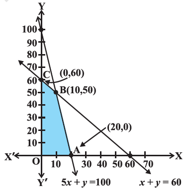
To dekho es graph ka jo shaded region hai that consists of the points common to all half planes determined by the inequalities. Each point in this region
represents a feasible choice open to the dealer for investing in tables and chairs. The region, therefore, is called the feasible region for the problem. Every point of this region is called a feasible solution to the problem. Thus, we the region OABC (shaded) is the feasible region for the problem. The region other than feasible region is called an infeasible region.
Optimal (feasible) solution : Any point in the feasible region that gives the optimal value (maximum or minimum) of the objective function is called an optimal solution.
To dekho ab humne dekha har ek point feasible region OABC ka satisfy karta hai sabhi constraints ko given in (1) to (4), to jaisa ki yha infinitely bahut se points hai, it is not evident how we should go about finding a point that gives a maximum value of the objective function Z=250x+75y. So, to handle this situation, we use the following theorems which are fundamental in solving linear programming problems. The proofs of these theorems are beyond the scope of the syllabus.
Theorem 1 : Let R be the feasible region (convex polygon) for a linear programming problem and let Z=ax+by be the objective function. When Z has an optimal value (maximum or minimum), where the variables x and y are subject to constraints described by linear inequalities, this optimal value must occur at a corner point (vertex) of the feasible region.
Theorem 2 : Let R be the feasible region for a linear programming problem, and let Z=ax+by be the objective function. If R is bounded, then the objective function Z has both a maximum and a minimum value on R and each of these occurs at a corner point (vertex) of R.
Corner Point
A corner point of a feasible region is a point in the region which is the intersection of two boundary lines.
We observe that the maximum profit to the dealer results from the investment strategy (10,50), i.e. buying 10 tables and 50 chairs.
This method of solving linear programming problem is referred as Corner Point
Method. The method comprises of the following steps :
1. Find the feasible region of the linear programming problem and determine its corner points (vertices) either by inspection or by solving the two equations of the lines intersecting at that point.
2. Evaluate the objective function Z=ax+by at each corner point. Let M and m,
respectively denote the largest and smallest values of these points.
3. (i) When the feasible region is bounded, M and m are the maximum and minimum values of Z.
(ii) In case, the feasible region is unbounded, we have :
4. (a)M is the maximum value of Z, if the open half plane determined by
ax+by>M has no point in common with the feasible region. Otherwise, Z has no maximum value.
(b) Similarly, m is the minimum value of Z, if the open half plane determined by ax+by<m has no point in common with the feasible region. Otherwise, Z has no minimum value.
We will now illustrate these steps of Corner Point Method by considering some examples :
Example 1
Draw the graph of the solution set of the system of inequations 2x+3y≤4,x≥0andy≥0.
Consider the equations
2x+3y=6,x+4y≤4,x=0andy=0.
Now, 2x+3y=63⇒x3+y2=1.
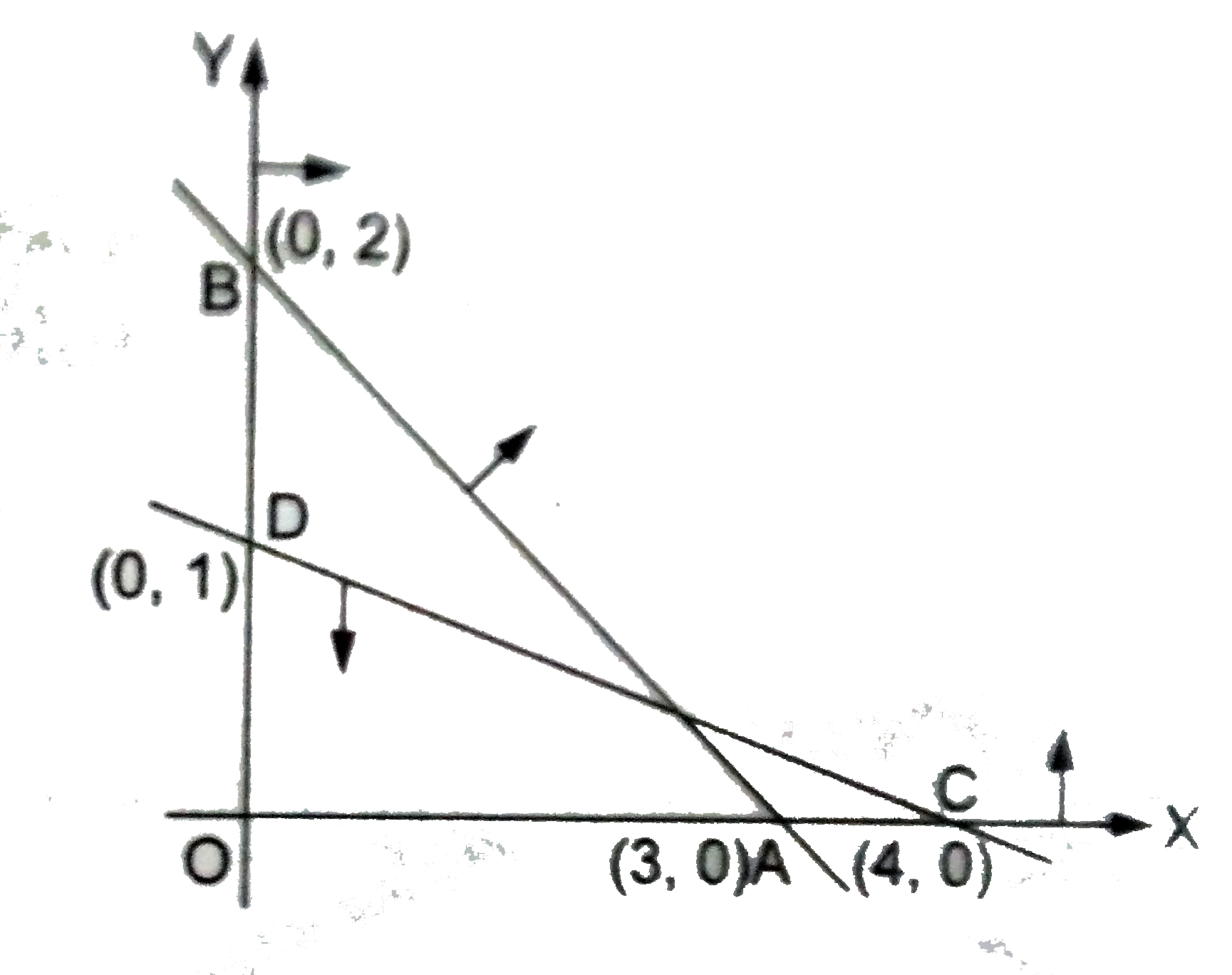
This line meets the axes at A(3,0)andB(0,2). Join these points and draw a thick line. Clearly, the portion not containing (0,0) represents the solution set of the inequation 2x+3y≥6. Again, x+4y=4⇒x4+y1=1.
This line meets the axes at C(4,0)andD(0,1). Join these points and draw a tick line. Clearly the portion containing (0,0) represents the solution set of the inequation x+4y≤4.
Clearly, x≥0 is represented by the y-axis and the portion on its right-hand side.
Also, y≥0 is represented by the x-axis and the portion above the x-axis.
Hence, the shaded region represents the solution set of the given inequations.
Example 2
Graph the solution set of the inequation 2x−y≥1.
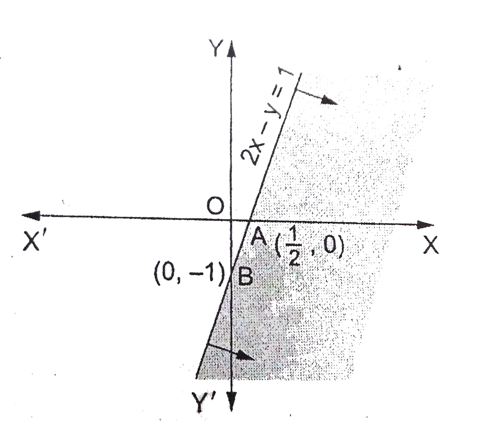
Consider the equation 2x−y=1.
We may write it as x(1/2)+y−1=1.
This shows that the line 2x−y=1 make intercepts of 12 and −1 on the axes.
Thus, the line meets the x-axis at A(12,0) and the y-axis at B(0,−1).
We plot these points and join them by a thick line Consider O(0,0). Clearly, (0,0) does not satisfy the given inequation. So, out of the portions divided by this line, the one not containing O(0,0) together with the points on the line, forms the solution set.
Example 3
Solve the following problem graphically :
Minimize and Maximize Z=3x+9y ...(1)
subject to the constraints: x+3y≤60 ...(2)
x+y≥10 ...(3)
x≤y ...(4)
x≥0,y≥0 . . . (5)
Region represented by x+3y≤60
Consider the equation x+3y=60.
x=0⇒3y=60⇒y=20,y=0⇒x=60
Plot the points A(2,20) and B(60,0). Join AB and produce it both ways.
Putting x=0 and y=0. we get 0+3×0=0≤60.
∴O(0,0) line in the region x+3y≤60.
So, the region containing the origin is the solution set of x+3y≥60.
Region represented by x+y≥10
Consider the equation x+y=10.
Plot the points C(0,10) and D(10,0). Join CD and product it both ways.
Now, x=0,y=0⇒0+0≥10 is not true.
∴O(0,0) lies in the region x−y≤0.
We know that:
x≥0 is the y-axis and the region on its RHS.
y≥0 is the x-axis and the region above the x-axis.
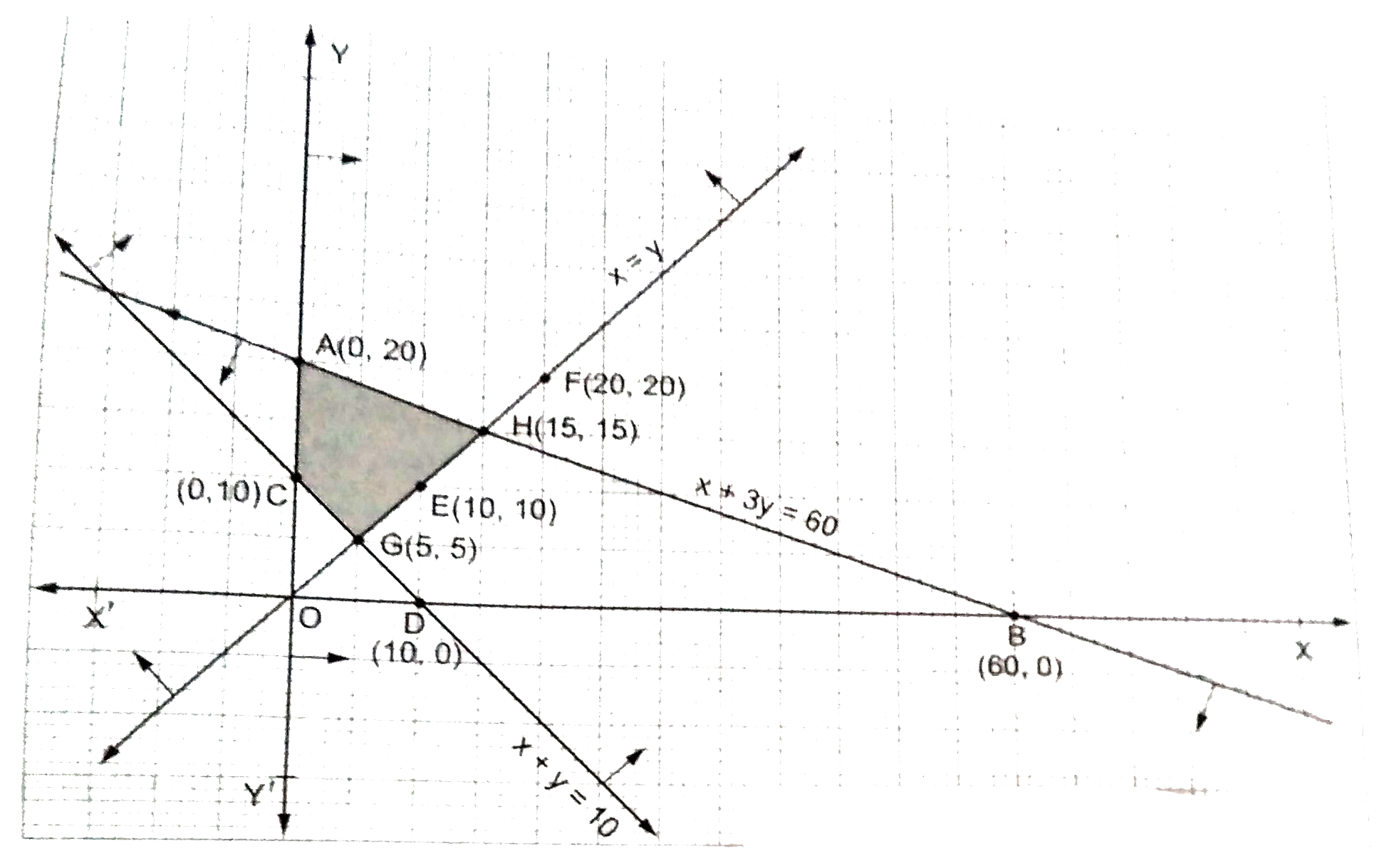
On solving x=yandx+y=10, we get the point G(5,5).
On solving x=yandx+3y=60, we get H(15,15).
Thus, the feasible region is ACGH, as shown in the figure.
Value of z=3x+9y:
(i)AtA(0,20)it is(3×0+9×20)=180.
(ii)AtC(0,10)it is(3×0+9×10)=90.
(iii)AtC(5,5)it is(3×5+9×10)=60.
(iii)AtH(15,15)it is(3×15+9×15)=180.
So the minimum value of z is 60 and its maximum value is 180.
Example 4
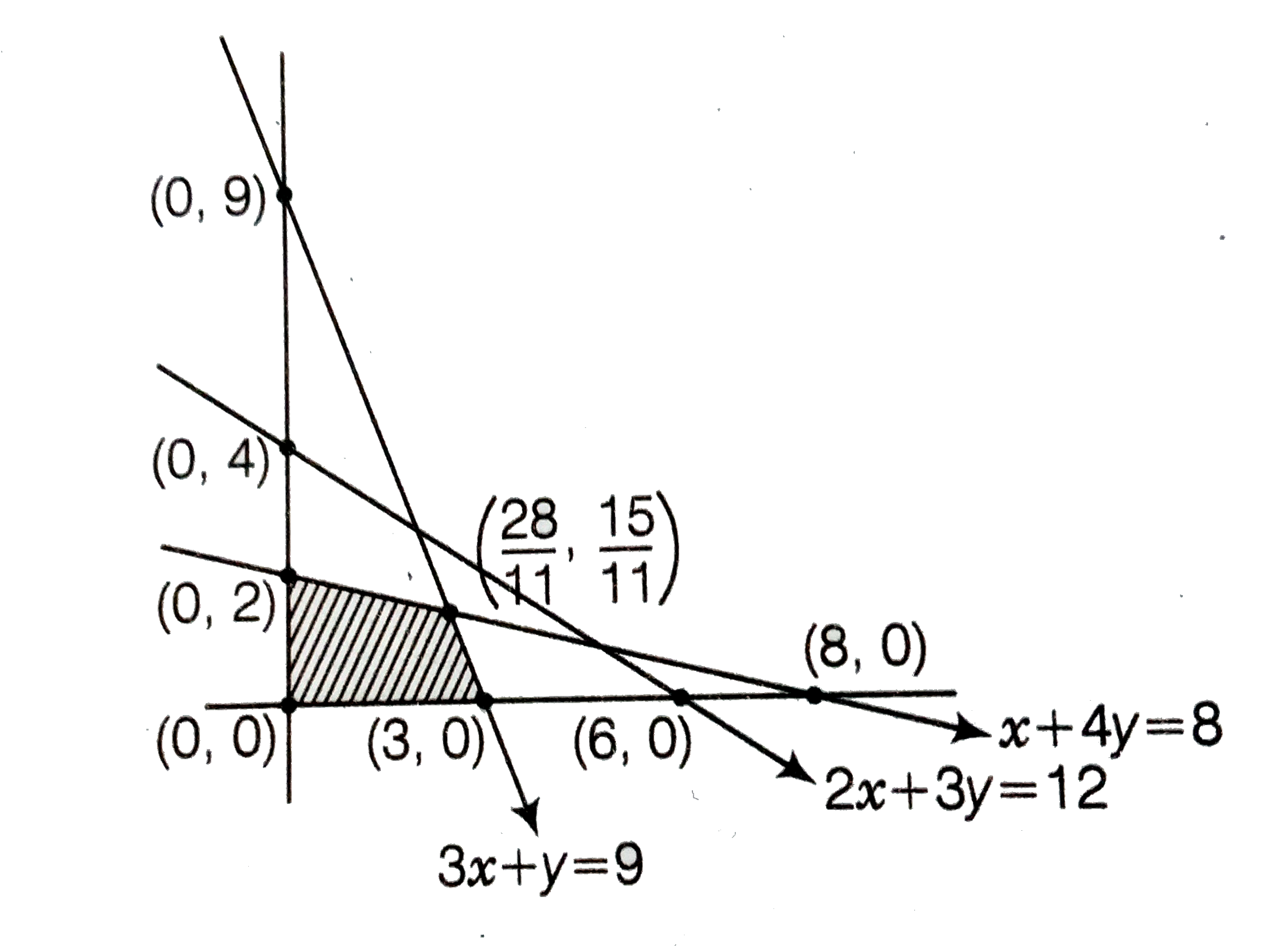
Maximize Z=x+y subject to x+4y≤8,2x+3y≤12,3x+y≤9,x≥0,andy≥0
Here the given LPP is
Maximize Z=X+Y subject to
x+4y≥8,2x+3y≤12,3x+y≤9,x≥0,y≥0
On solving x+4y=8 and 3x+y=9 we get
x=2811,y=1511
From the feasible region, it is clear that coordinates of corner points are (0,0),(3,0),(2811,1511) and (0,2)
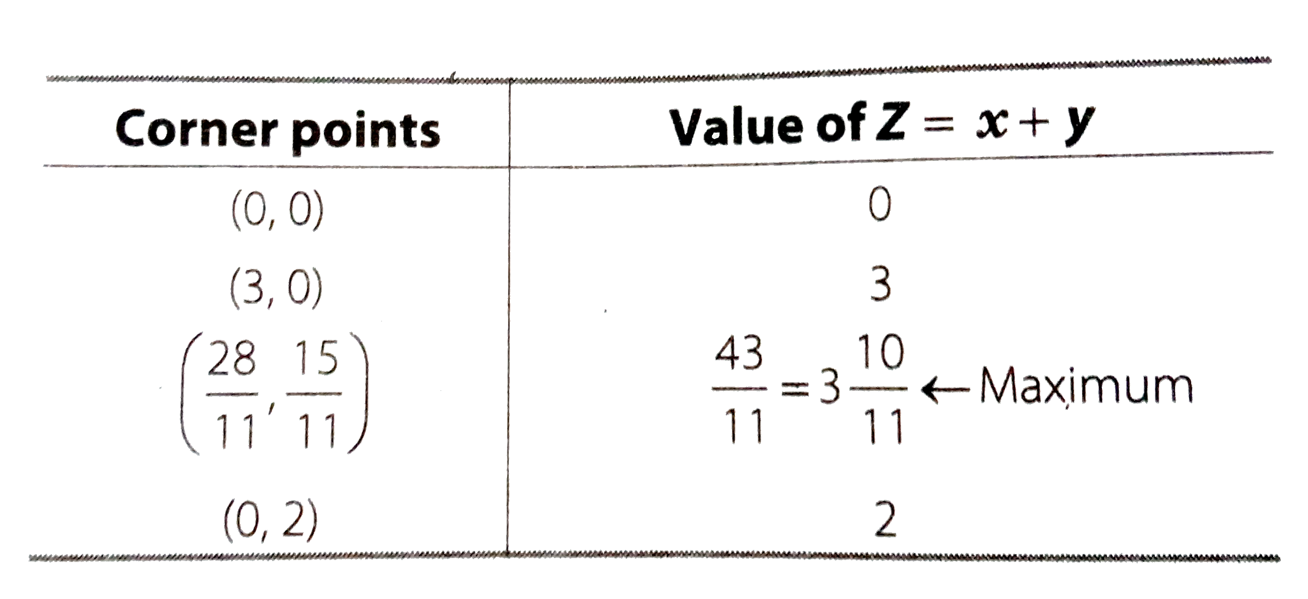
Hence, the maximum value is 31011
Different Types of Linear Programming Problems
A few important linear programming problems are listed below :
1. Manufacturing problems : Es tarh ki problems mein hum number of units nikalte hai different products ki jo ki ek firm ke through produce ki jati hai aur bechi jati hai. Basically product mein hone vala sara kharch karne ke baad maximum profit nikalne ke liye. Like each product requires a fixed manpower, machine hours, labour hour per
unit of product, warehouse space per unit of the output etc.
2. Diet problems : En problems mein hum determine karte hai amount of different kinds of constituents/nutrients which should be included in a diet so as to minimize the
cost of the desired diet such that it contains a certain minimum amount of each
constituent/nutrients.
3. Transportation problems : En problems mein hum determine karte hai a transportation
schedule in order to find the cheapest way of transporting a product from
plants/factories situated at different locations to different markets.
Example 5
A firm manufactures two types of products, A and B, and sells them at a profit of 3 per unit of type B product and 5 per unit of type A product. Both product is processed on two machines M1 and M2. One unit of type A requires one minute of processing time on M1 and two minutes of processing time on M2 whereas one unit of type B requires one minute of processing time on M1 and one minute on M2 Machines. M1, and M2, are respectively available for at most 5 hours and 6 hours in a day. Find out how many units of each type of product the firm should produce a day in order to maximize the profit. Solve the problem graphically.
Let x units of A and y units of B be produced in order to have a maximum profit.
Then, clearly x≥0 and y≥0. x unit of A and y units of B will take (x+y) minutes on M1.
∴x+y≤300.
x units of A and y units of B will take (2x+y) minutes on M2.∴2x+y≤360.
Let Z be the profit function. Then Z=5x+3y.
We have to maximize Z=5x+3y, subject to the constraints
x≥0,y≥0,x+y≤300and2x+y≤360.
Now, x+y=300⇒x300+y300=1.
This line meets the axes in (300,0)and(0,300).
Joining these points, we get line x+y=300.
Since (0,0) satisfies the inequation x+y≤300, the region below the line x+y=300 containing O(0,0) represents x+y≤300.
Again, 2x+y=360⇒x180+y360=1.
This line meets the axis in (180,0)and(0,360).
Joining these points, we get the line 2x+y=360.
Since (0,0) satisfies 2x+y≤360, the region below the line 2x+y=360 containing (0,0) represents 2x+y≤360.
Also x=0 is the y-axis and y=0 is the x-axis.
On drawing these lines and shading the feasible region, we obtain a figure, given below.
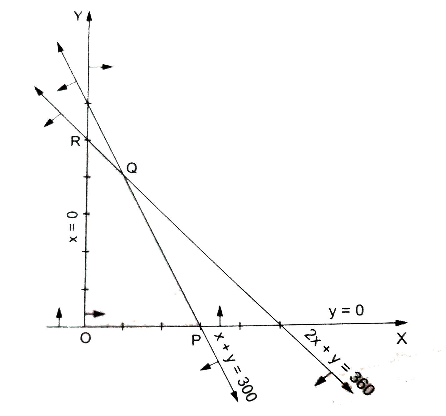
On solving x+y=300 and
2x+y=360, we get the point Q(60,240). ∴ the vertices of the feasible region are
O(0,0),P(180,0),Q(60,240)andR(0,300).
Values of Z=5x+3y at O,P,Q,R are 0,900,1020,900 respectively.
∴ Z is maximum when x=60 and y=240.
Example 6
If a young man rides his motorcycle at 25 km/hr, he has to spend Rs. 2 per kilometer on petrol. If he rides it at a faster speed of 40 km/hr the petrol cost increases to Rs. 5 per kilometer. He has Rs. 100 to spend on petrol and wishes to find the maximum distance he can travel within one hour. Express this as an LPP and solve it. graphically.
Let us assume that the man travels x km when the speed is 25 km/h and y km when the speed is 40 km/h.
Thus, the total distance travelled is given by P=x+y km and we have to maximize it.
Clearly, x≥0,2x+5y≤100.
Since the available time is at most one hour, we have
x25+y40≤1 or 8x+5y≤200.
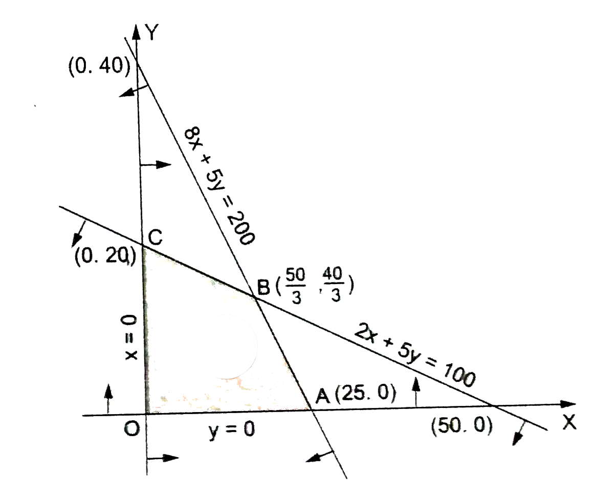
Now, we solved the system of the inequations.
2x+5y=100⇒x50+y20=1.
This line meets the axes at (50,0) and
(0,20). Plot these points and join them to get the line 2x+5y=100.
Also, 8x+5y=200⇒x25+y40=1.
This line meets the axes at (25,0) and (0,40). Plot these points and obtain the line 8x+5y=200.
x=0 is the y-axis and y=0 is the x-axis.
We find that the solution set of the above system is the shaded region OABC.
The coordinates of O,A,B,C are (0,0),(25,0),(503,403) and (0,20) respectively.
So, P=x+y is maximum when x=503 and y=403.
Thus the young man can cover the maximum distance of 30 km, if he rides 503 km/h and 403 km at 40 km/h.
Summary
- A linear programming problem is one that is concerned with finding the optimal value (maximum or minimum) of a linear function of several variables (called objective function) subject to the conditions that the variables are non-negative and satisfy a set of linear inequalities (called linear constraints). Variables are sometimes called decision variables and are non-negative.
- A few important linear programming problems are :
(i) Diet problems
(ii) Manufacturing problems
(iii) Transportation problems - The common region determined by all the constraints including the non-negative constraints x≥0, y≥0 of a linear programming problem is called the feasible region (or solution region) for the problem.
- Points within and on the boundary of the feasible region represent feasible solutions of the constraints. Any point outside the feasible region is an infeasible solution.
- Any point in the feasible region that gives the optimal value (maximum or minimum) of the objective function is called an optimal solution.
- The following Theorems are fundamental in solving linear programming
problems :
Theorem 1 Let R be the feasible region (convex polygon) for a linear programming problem and let Z=ax+by be the objective function. When Z has an optimal value (maximum or minimum), where the variables x and y are subject to constraints described by linear inequalities, this optimal value must occur at a corner point (vertex) of the feasible region. - Theorem 2 Let R be the feasible region for a linear programming problem, and let Z=ax+by be the objective function. If R is bounded, then the objective function Z has both a maximum and a minimum value on R and each of these occurs at a corner point (vertex) of R.
- If the feasible region is unbounded, then a maximum or a minimum may not exist However, if it exist, it must occur at a corner point of R.
- Corner point method for solving a linear programming problem. The method
comprises of the following steps :
(i) Find the feasible region of the linear programming problem and determine its corner points (vertices).
(ii) Evaluate the objective function Z=ax+by at each corner point. Let M and m respectively be the largest and smallest values at these points.
(iii) If the feasible region is bounded, M and m respectively are the maximum and minimum values of the objective function.
If the feasible region is unbounded, then
(i) M is the maximum value of the objective function, if the open half plane determined by ax+by>M has no point in common with the feasible region. Otherwise, the objective function has no maximum value.
(ii) m is the minimum value of the objective function, if the open half plane determined by ax+by<m has no point in common with the feasible region. Otherwise, the objective function has no minimum value. - If two corner points of the feasible region are both optimal solutions of the same type, i.e., both produce the same maximum or minimum, then any point on the line segment joining these two points is also an optimal solution of the same type.
Let's Revise
- To bachcho ab hum Linear programming chapter ka quick revision karenge.
- Linear programming problems provide the method of finding an optimized function along with the values which would optimize the required function.
- Formulation of LPP
Step (1) : Identify the number of decision variables which govern the behaviour of objective function.
Step (2) : Identify the set of constraints on the decision variables and express them in the form of linear inequations or linear equations.
Step (3) : Express the objective function in the form of a linear equation in the decision variable.
Step (4) : Optimize the objective function either graphically or mathematically.
Types of LPP
| Type of LPP | Constraints | Objective Function |
|---|---|---|
| Diet Problems | The specified nutritional requirement | The cost of food Intake |
| Manufacturing Problems | Variables like work hour, material availability, production rate, etc. | The cost of production |
| Transportation Problems | The specific supply demand pattern | The cost of transportation |
| Optimal Assignment Problems | The number of employees, work hour of each employee, efficiency of employee, etc. | The total assignment done |