A rod of length L and uniform cross-sectional area has varying thermal conductivity which changes linearly from 2K at end A to K at the other end B. The ends A and B of the rod are maintained at constant temperture 100∘C and 0∘C, respectively. At steady state, the graph of temperture : T=T(x) where x= distance from end A will be
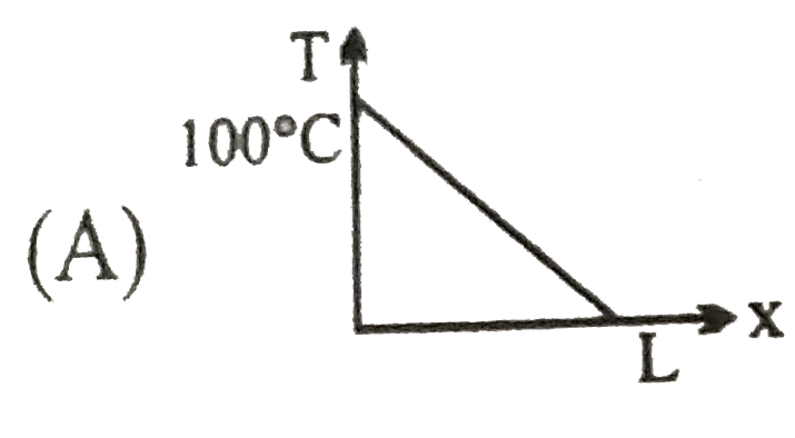
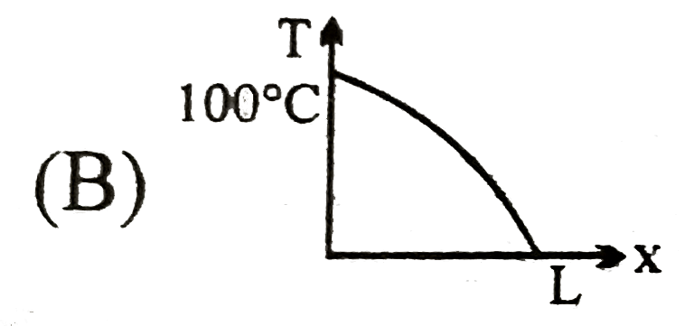
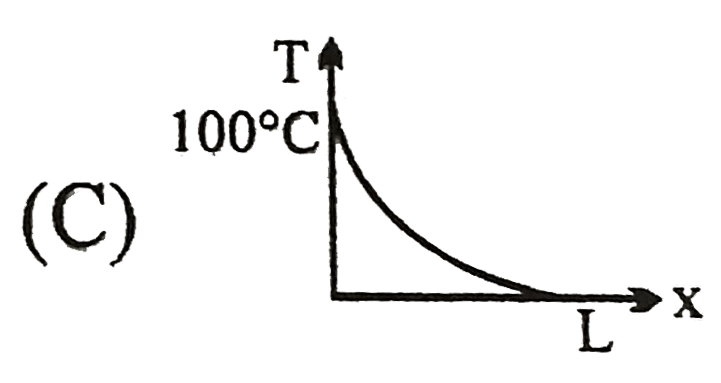
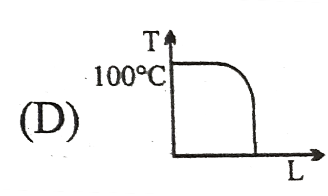
To solve the problem, we need to analyze the heat transfer through a rod with varying thermal conductivity. Here’s a step-by-step breakdown of the solution:
Step 1: Understand the Problem
We have a rod of length L with thermal conductivity that varies linearly from 2K at one end (A) to K at the other end (B). The temperatures at the ends are maintained at 100°C (at A) and 0°C (at B). We need to find the temperature distribution T(x) along the length of the rod.
Step 2: Define the Thermal Conductivity as a Function of Position
Since the thermal conductivity changes linearly, we can express it as:
\( K(x) = K_A + \left( \frac{K_B - K_A}{L} \right) x \)
Where:
- \( K_A = 2K \) (at A)
- \( K_B = K \) (at B)
Thus, we can write:
\( K(x) = 2K - \frac{K}{L} x \)
Step 3: Apply Fourier's Law of Heat Conduction
According to Fourier's law, the rate of heat transfer \( I \) through the rod can be expressed as:
\( I = -K(x) A \frac{dT}{dx} \)
Where:
- \( A \) is the cross-sectional area (assumed constant).
Step 4: Substitute \( K(x) \) into Fourier's Law
Substituting \( K(x) \) into the equation gives:
\( I = -\left(2K - \frac{K}{L} x\right) A \frac{dT}{dx} \)
Step 5: Rearranging the Equation
Rearranging the equation to isolate \( \frac{dT}{dx} \):
\( \frac{dT}{dx} = -\frac{I}{A} \cdot \frac{1}{2K - \frac{K}{L} x} \)
Step 6: Integrate the Equation
To find the temperature distribution, we need to integrate:
\( \int dT = -\int \frac{I}{A} \cdot \frac{1}{2K - \frac{K}{L} x} dx \)
Step 7: Solve the Integral
This integral can be solved using the natural logarithm:
\( T(x) - T_1 = -\frac{IL}{K} \ln\left(2K - \frac{K}{L} x\right) + C \)
Where \( T_1 \) is the temperature at \( x = 0 \) (which is \( 100°C \)).
Step 8: Apply Boundary Conditions
Using the boundary conditions:
1. At \( x = 0 \), \( T = T_1 = 100°C \)
2. At \( x = L \), \( T = T_2 = 0°C \)
Step 9: Final Equation for Temperature Distribution
After applying the boundary conditions, we can express the final equation for temperature as:
\( T(x) = T_1 - \frac{IL}{K} \ln\left(\frac{2K - \frac{K}{L} x}{K}\right) \)
Step 10: Analyze the Graph of \( T(x) \)
1. The graph of \( T \) versus \( x \) will be decreasing since \( dT/dx < 0 \).
2. The second derivative \( d^2T/dx^2 \) will be positive, indicating that the graph is concave upward.
Conclusion
The graph of temperature \( T \) as a function of distance \( x \) from end A will be a decreasing curve that is concave upward.
We have a rod of length L with thermal conductivity that varies linearly from 2K at one end (A) to K at the other end (B). The temperatures at the ends are maintained at 100°C (at A) and 0°C (at B). We need to find the temperature distribution T(x) along the length of the rod.
Since the thermal conductivity changes linearly, we can express it as:
\( K(x) = K_A + \left( \frac{K_B - K_A}{L} \right) x \)
Where:
- \( K_A = 2K \) (at A)
- \( K_B = K \) (at B)
\( K(x) = 2K - \frac{K}{L} x \)
According to Fourier's law, the rate of heat transfer \( I \) through the rod can be expressed as:
\( I = -K(x) A \frac{dT}{dx} \)
Where:
- \( A \) is the cross-sectional area (assumed constant).
Substituting \( K(x) \) into the equation gives:
\( I = -\left(2K - \frac{K}{L} x\right) A \frac{dT}{dx} \)
Rearranging the equation to isolate \( \frac{dT}{dx} \):
\( \frac{dT}{dx} = -\frac{I}{A} \cdot \frac{1}{2K - \frac{K}{L} x} \)
To find the temperature distribution, we need to integrate:
\( \int dT = -\int \frac{I}{A} \cdot \frac{1}{2K - \frac{K}{L} x} dx \)
This integral can be solved using the natural logarithm:
\( T(x) - T_1 = -\frac{IL}{K} \ln\left(2K - \frac{K}{L} x\right) + C \)
Where \( T_1 \) is the temperature at \( x = 0 \) (which is \( 100°C \)).
Using the boundary conditions:
1. At \( x = 0 \), \( T = T_1 = 100°C \)
2. At \( x = L \), \( T = T_2 = 0°C \)
After applying the boundary conditions, we can express the final equation for temperature as:
\( T(x) = T_1 - \frac{IL}{K} \ln\left(\frac{2K - \frac{K}{L} x}{K}\right) \)
1. The graph of \( T \) versus \( x \) will be decreasing since \( dT/dx < 0 \).
2. The second derivative \( d^2T/dx^2 \) will be positive, indicating that the graph is concave upward.
The graph of temperature \( T \) as a function of distance \( x \) from end A will be a decreasing curve that is concave upward.
Topper's Solved these Questions
Similar Questions
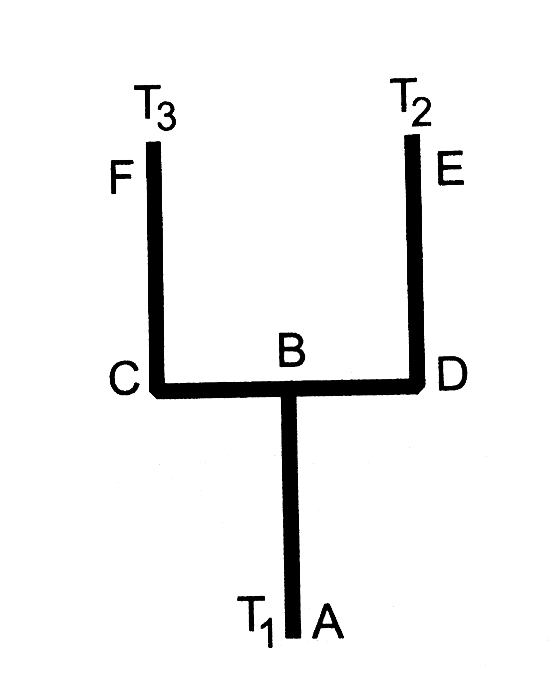
Four identical rods AB, CD, CF and DE are joined as shown in figure. The length, cross-sectional area and thermal conductivity of each rod are l, A and K respectively. The ends A, E and F are maintained at temperature T1 , T2 and T3 respectively. Assuming no loss of heat to the atmospere, find the temperature at B.
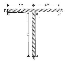
View SolutionTwo identical rods AB and CD, each of length L are connected as shown in figure-4.22. Their cross-sectional area is A and their thermal conductivity is k. Ends A, C and D are maintained at temperatures T1,T2andT3 respectively. Neglecting heat loss to the surroundings, find the temperature at B.
View Solution
Knowledge Check
Two ends of a conducting rod of varying cross-section are maintained at 200∘Cand0∘C respectively. In steady state :
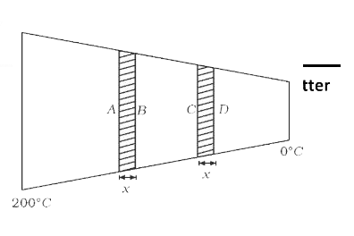 Atemperature differences across AB and CD are equalBtemperature difference across AB is greater than that across CDCtemperature difference across AB is less than that across CDDtemperature difference may be equal or different depending upon thermal conductivity of the rod.
Two ends of a conducting rod of varying cross-section are maintained at 200∘C and 0∘C respectively. In steady state:
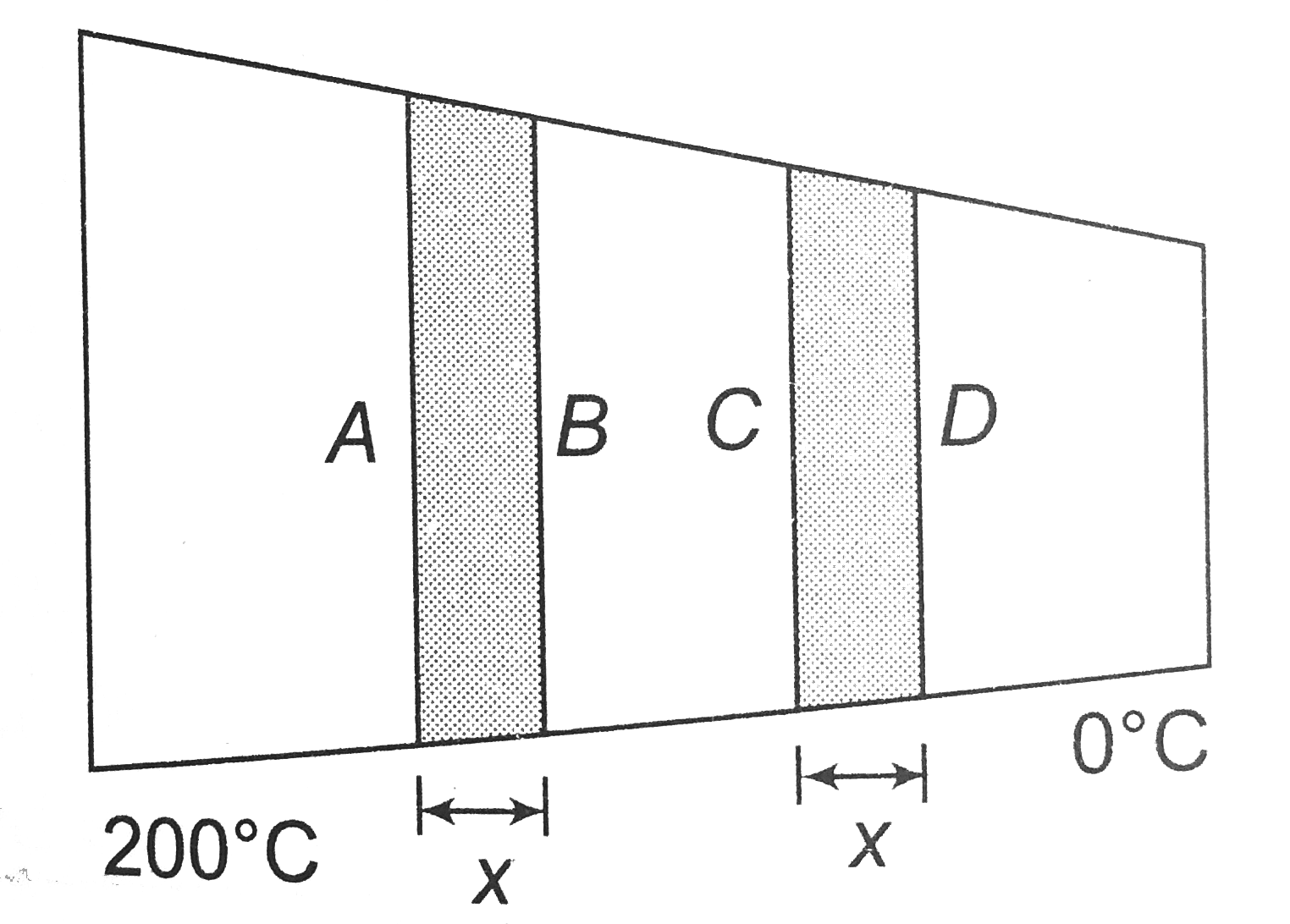 Atemperature differences across ABandCD are equalBtemperature difference aross AB is greater than that across CDCtemperature difference aross AB is less than that across CDDtemperature difference may be equal or different depending upon thermal conductivity of the rod.
The ends of a rod of uniform thermal conductivity are maintained at different (constant) temperatures. Afer the steady state is achieved:
Aheat flows in the rod from high temperature to low temperature even if the rod has nonuniform cross sectional area.Btemperature gradient along length is same even if the rod has non uniform cross sectional area.Cheat current is same even if the rod has nono-uniform cross sectional areaDif the rod has uniform cross sectional area the temperature is same at all points of the rod.
The temperature of the two ends A and B of a rod of length 25cm and circular cross section are 100∘C and 0∘C respectively In the steady state, find the temperature at a point 10cm from the end B (ifnore loss of heat from curved surface of the body) ?
View SolutionA rod of length l and cross-section area A has a variable thermal conductivity given by K = α T, where α is a positive constant and T is temperature in kelvin. Two ends of the rod are maintained at temperature T1 and T2 (T1>T2). Heat current flowing through the rod will be
View SolutionIn a steady state of thermal conduction, temperature of the ends A and B of a 20 cm long rod are 100∘C and 0∘C respectively. What will be the temperature of the rod at a point at a distance of 6 cm from the end A of the rod
View SolutionA rod of length l and cross sectional area A has a variable conductivity given by K=αT, where α is a positive constant T is temperatures in Kelvin. Two ends of the rod are maintained at temperatures T1 and T2(T1>T2). Heat current flowing through the rod will be
View SolutionThe temperature of hot and cold end of a 20 cm long rod in thermal steady state are at 100∘C and 20∘C respectively. Temperature at the centre of the rod is
View Solution